서울시 상권매출 데이터 다중회귀분석/군집분석 프로젝트
사실 이건 수업에서 프로젝트로 해볼 예정이었는데 엎어지는 바람에 제가 진행해본 부분만을 정리하려 합니다.
그렇기에 부족한 부분이 있을 수 있다는 점을 감안해주시면 감사하겠습니다. 😊
https://data.seoul.go.kr/dataList/OA-15572/S/1/datasetView.do
데이터는 서울시 열린 데이터 광장에서 가져왔습니다.
서울시 우리 마을가게 상권분석 서비스(상권-추정 매출) 데이터이며, 2021년 데이터만 가져왔습니다.
요일별, 시간대별, 연령대 등등 세부적으로 매출을 확인할 수 있습니다.
저는 이러한 세부적인 매출을 통해 총매출을 예측하는 다중회귀모델을 찾아내고, 업종을 3가지로 구분해 각 업종별로 군집분석을 하는 것을 큰 주제로 정하려 합니다.
import numpy as np
import pandas as pd
import matplotlib.pyplot as plt
import seaborn as sns
import warnings
warnings.filterwarnings('ignore')
pd.set_option('display.max_columns', None)
pd.set_option('display.max_rows', None)
# 한글 폰트 적용
from matplotlib import font_manager, rc
font_name = font_manager.FontProperties(fname = "c:/Windows/Fonts/malgun.ttf").get_name()
rc('font', family = font_name)필요한 라이브러리를 불러옵니다.
df2021=pd.read_csv(r'C:\Users\서울시우리마을가게상권분석서비스(상권-추정매출)_2021 (1)\서울시 우리마을가게 상권분석서비스(상권-추정매출)2.csv',encoding='UTF-8')
df2021.info()<class 'pandas.core.frame.DataFrame'>
RangeIndex: 128703 entries, 0 to 128702
Data columns (total 80 columns):
# Column Non-Null Count Dtype
--- ------ -------------- -----
0 기준_년_코드 128703 non-null int64
1 기준_분기_코드 128703 non-null int64
2 상권_구분_코드 128703 non-null object
3 상권_구분_코드_명 128703 non-null object
4 상권_코드 128703 non-null int64
5 상권_코드_명 128703 non-null object
6 서비스_업종_코드 128703 non-null object
7 서비스_업종_코드_명 128703 non-null object
8 분기당_매출_금액 128703 non-null float64
9 분기당_매출_건수 128703 non-null int64
10 주중_매출_비율 128703 non-null int64
11 주말_매출_비율 128703 non-null int64
12 월요일_매출_비율 128703 non-null int64
13 화요일_매출_비율 128703 non-null int64
14 수요일_매출_비율 128703 non-null int64
15 목요일_매출_비율 128703 non-null int64
16 금요일_매출_비율 128703 non-null int64
17 토요일_매출_비율 128703 non-null int64
18 일요일_매출_비율 128703 non-null int64
19 시간대_00~06_매출_비율 128703 non-null int64
20 시간대_06~11_매출_비율 128703 non-null int64
21 시간대_11~14_매출_비율 128703 non-null int64
22 시간대_14~17_매출_비율 128703 non-null int64
23 시간대_17~21_매출_비율 128703 non-null int64
24 시간대_21~24_매출_비율 128703 non-null int64
25 남성_매출_비율 128703 non-null int64
26 여성_매출_비율 128703 non-null int64
27 연령대_10_매출_비율 128703 non-null int64
28 연령대_20_매출_비율 128703 non-null int64
29 연령대_30_매출_비율 128703 non-null int64
30 연령대_40_매출_비율 128703 non-null int64
31 연령대_50_매출_비율 128703 non-null int64
32 연령대_60_이상_매출_비율 128703 non-null int64
33 주중_매출_금액 128703 non-null float64
34 주말_매출_금액 128703 non-null float64
35 월요일_매출_금액 128703 non-null int64
36 화요일_매출_금액 128703 non-null int64
37 수요일_매출_금액 128703 non-null int64
38 목요일_매출_금액 128703 non-null int64
39 금요일_매출_금액 128703 non-null int64
40 토요일_매출_금액 128703 non-null int64
41 일요일_매출_금액 128703 non-null int64
42 시간대_00~06_매출_금액 128703 non-null int64
43 시간대_06~11_매출_금액 128703 non-null int64
44 시간대_11~14_매출_금액 128703 non-null float64
45 시간대_14~17_매출_금액 128703 non-null float64
46 시간대_17~21_매출_금액 128703 non-null int64
47 시간대_21~24_매출_금액 128703 non-null int64
48 남성_매출_금액 128703 non-null float64
49 여성_매출_금액 128703 non-null float64
50 연령대_10_매출_금액 128703 non-null int64
51 연령대_20_매출_금액 128703 non-null int64
52 연령대_30_매출_금액 128703 non-null int64
53 연령대_40_매출_금액 128703 non-null float64
54 연령대_50_매출_금액 128703 non-null int64
55 연령대_60_이상_매출_금액 128703 non-null int64
56 주중_매출_건수 128703 non-null int64
57 주말_매출_건수 128703 non-null int64
58 월요일_매출_건수 128703 non-null int64
59 화요일_매출_건수 128703 non-null int64
60 수요일_매출_건수 128703 non-null int64
61 목요일_매출_건수 128703 non-null int64
62 금요일_매출_건수 128703 non-null int64
63 토요일_매출_건수 128703 non-null int64
64 일요일_매출_건수 128703 non-null int64
65 시간대_건수~06_매출_건수 128703 non-null int64
66 시간대_건수~11_매출_건수 128703 non-null int64
67 시간대_건수~14_매출_건수 128703 non-null int64
68 시간대_건수~17_매출_건수 128703 non-null int64
69 시간대_건수~21_매출_건수 128703 non-null int64
70 시간대_건수~24_매출_건수 128703 non-null int64
71 남성_매출_건수 128703 non-null int64
72 여성_매출_건수 128703 non-null int64
73 연령대_10_매출_건수 128703 non-null int64
74 연령대_20_매출_건수 128703 non-null int64
75 연령대_30_매출_건수 128703 non-null int64
76 연령대_40_매출_건수 128703 non-null int64
77 연령대_50_매출_건수 128703 non-null int64
78 연령대_60_이상_매출_건수 128703 non-null int64
79 점포수 128703 non-null int64
dtypes: float64(8), int64(68), object(5)
memory usage: 79.5+ MB총 80개의 칼럼이 존재하며, 결측치는 없는 것으로 확인됩니다.
간단하게 칼럼들을 확인해보겠습니다.
plt.figure(figsize=(10,5))
sns.countplot(x=df2021['상권_구분_코드_명'])
상권 구분 코드별로 값의 개수 차이가 많이 나는 것을 볼 수 있었습니다. 골목상권의 데이터가 가장 많으며, 관광특구의 데이터는 매우 적었습니다.
다음으로 서비스 업종별 점포수를 확인하려 합니다.
상권 매출 데이터에서 하나의 행은 상권 구분 코드, 서비스 업종 코드가 같은 서비스 업종을 모아 매출을 나타낸 것입니다. (아마 하나의 행이 하나의 매장을 의미하면 각 매장의 매출이 드러나게 되어 이렇게 모아놓은 듯합니다.)
그렇기에 점포수를 파악하려면 행의 개수가 아닌, 점포수 칼럼을 사용해야 합니다.
service=df2021.groupby('서비스_업종_코드_명').agg({'기준_년_코드':'count', '점포수':sum},as_index=False).reset_index()
service.columns=['서비스_업종','개수','점포수']
service=service.sort_values('점포수',ascending=False).iloc[:20]

plt.figure(figsize=(25,10))
sns.barplot(x=service['서비스_업종'],y=service['점포수'])
서비스 업종은 약 60개 정도가 있는 것으로 확인했는데, 이 60개를 모두 그래프에 나타내기엔 너무 많아 점포가 많은 업종 20개만 그래프로 나타내었습니다.

일반 의류, 한식 음식점의 점포수가 가장 많은 것을 확인할 수 있었습니다.
이제 매출 금액과 관련 있는 칼럼을 확인하기 위해 상관관계 그래프를 그려보겠습니다.
all=df2021[['분기당_매출_금액','분기당_매출_건수','주중_매출_금액','주말_매출_금액']].corr()
plt.figure(figsize=(10,10))
sns.heatmap(data = all.corr(), annot=True,
fmt = '.2f', linewidths=.5, cmap='Blues')
week=df2021[['분기당_매출_금액','월요일_매출_금액','화요일_매출_금액','수요일_매출_금액','목요일_매출_금액','금요일_매출_금액'
       ,'토요일_매출_금액','일요일_매출_금액']].corr()

plt.figure(figsize=(10,10))
sns.heatmap(data = week, annot=True,
fmt = '.2f', linewidths=.5, cmap='Blues')
time=df2021[['분기당_매출_금액','시간대_00~06_매출_금액','시간대_06~11_매출_금액','시간대_11~14_매출_금액'
            ,'시간대_14~17_매출_금액','시간대_17~21_매출_금액','시간대_21~24_매출_금액']].corr()

plt.figure(figsize=(10,10))
sns.heatmap(data = time, annot=True,
fmt = '.2f', linewidths=.5, cmap='Blues')
gender=df2021[['분기당_매출_금액','여성_매출_금액','남성_매출_금액']].corr()

plt.figure(figsize=(10,10))
sns.heatmap(data = gender, annot=True,
fmt = '.2f', linewidths=.5, cmap='Blues')
age=df2021[['분기당_매출_금액','연령대_10_매출_금액','연령대_20_매출_금액','연령대_30_매출_금액'
           ,'연령대_40_매출_금액','연령대_50_매출_금액','연령대_60_이상_매출_금액']].corr()

plt.figure(figsize=(10,10))
sns.heatmap(data = age, annot=True,
fmt = '.2f', linewidths=.5, cmap='Blues')
all2=df2021[['분기당_매출_금액','분기당_매출_건수','주중_매출_건수','주말_매출_건수','점포수']].corr()
plt.figure(figsize=(10,10))
sns.heatmap(data = all2.corr(), annot=True,
fmt = '.2f', linewidths=.5, cmap='Blues')
week2=df2021[['분기당_매출_금액','월요일_매출_건수','화요일_매출_건수','수요일_매출_건수','목요일_매출_건수','금요일_매출_건수'
       ,'토요일_매출_건수','일요일_매출_건수']].corr()

plt.figure(figsize=(10,10))
sns.heatmap(data = week, annot=True,
fmt = '.2f', linewidths=.5, cmap='Blues')
time2=df2021[['분기당_매출_금액','시간대_건수~06_매출_건수','시간대_건수~11_매출_건수','시간대_건수~14_매출_건수'
            ,'시간대_건수~17_매출_건수','시간대_건수~21_매출_건수','시간대_건수~24_매출_건수']].corr()

plt.figure(figsize=(10,10))
sns.heatmap(data = time2, annot=True,
fmt = '.2f', linewidths=.5, cmap='Blues')
gender=df2021[['분기당_매출_금액','여성_매출_건수','남성_매출_건수']].corr()

plt.figure(figsize=(10,10))
sns.heatmap(data = gender, annot=True,
fmt = '.2f', linewidths=.5, cmap='Blues')
age2=df2021[['분기당_매출_금액','연령대_10_매출_건수','연령대_20_매출_건수','연령대_30_매출_건수'
           ,'연령대_40_매출_건수','연령대_50_매출_건수','연령대_60_이상_매출_건수']].corr()

plt.figure(figsize=(10,10))
sns.heatmap(data = age2, annot=True,
fmt = '.2f', linewidths=.5, cmap='Blues')
특징별 매출, 건수와 총 매출금 액간의 상관관계를 그려보았습니다.
대부분의 칼럼이 총매출과 높은 상관관계를 나타내는 듯 보입니다. 저는 이 중에서 총매출과의 상관관계가 0.6 이상인 칼럼을 선택해 다중회귀분석을 해보려 합니다.
X=df2021[[ '분기당_매출_건수', '주중_매출_금액', '주말_매출_금액', '월요일_매출_금액',
       '화요일_매출_금액', '수요일_매출_금액', '목요일_매출_금액', '금요일_매출_금액', '토요일_매출_금액',
       '일요일_매출_금액', '시간대_06~11_매출_금액', '시간대_11~14_매출_금액',
       '시간대_14~17_매출_금액', '시간대_17~21_매출_금액', '남성_매출_금액',
       '여성_매출_금액', '연령대_20_매출_금액', '연령대_30_매출_금액',
       '연령대_40_매출_금액', '연령대_50_매출_금액', '연령대_60_이상_매출_금액',
       '토요일_매출_건수', '시간대_건수~17_매출_건수',
      '연령대_50_매출_건수']]

y=df2021['분기당_매출_금액']
총 24개의 칼럼이 선택되었으며, 다중회귀분석 시 칼럼명이 한글이면 인식을 못하는 것 같아 영어로 칼럼명을 바꿔주었습니다.
X.columns=[['cnt','weekday_amt','weekend_amt','mon_amt','tue_amt','wed_amt','thu_amt','fri_amt','sat_amt','sun_amt','0611_amt','1114_amt',
           '1417_amt','1721_amt','man_amt','woman_amt','20_amt','30_amt','40_amt','50_amt','60_amt','sat_cnt','1417_cnt','50_cnt']]
다중회귀분석을 들어가기 전, 회귀분석에서는 종속변수 간의 상관관계가 분석에 좋지 않은 영향을 줍니다. 이를 다중공선성이라고 합니다.
다중공선성이 있을 경우, 제거를 해야 하기에 있는지 확인해보았습니다.
from patsy import dmatrices
import statsmodels.api as sm
from statsmodels.stats.outliers_influence import variance_inflation_factor
pd.options.display.float_format = '{:.5f}'.format
vif=pd.DataFrame()
vif['features']=[variance_inflation_factor(X.values,i) for i in range(X.shape[1])]
vif['VIF Factor']=X.columns
vif=vif.sort_values('features').reset_index(drop=True)
vif VIF Factor features
0 13.72073 (0611_amt,)
1 32.46843 (1114_amt,)
2 46.96941 (1417_amt,)
3 24.10502 (1417_cnt,)
4 29.04975 (1721_amt,)
5 1449.89886 (20_amt,)
6 2911.47573 (30_amt,)
7 6050.09918 (40_amt,)
8 4577.17843 (50_amt,)
9 21.11021 (50_cnt,)
10 4832.83708 (60_amt,)
11 27.39866 (cnt,)
12 39494866503.29296 (fri_amt,)
13 24298.48908 (man_amt,)
14 29311150339.54556 (mon_amt,)
15 417754243993.36731 (sat_amt,)
16 22.76129 (sat_cnt,)
17 180885616120.91559 (sun_amt,)
18 33317055257.44963 (thu_amt,)
19 28795117868.88550 (tue_amt,)
20 31721410174.22615 (wed_amt,)
21 780790504051.75037 (weekday_amt,)
22 1105449098520.00391 (weekend_amt,)
23 16580.14830 (woman_amt,)보통 10 이상이면 다중공선성이 있다고 판단하는데 모든 변수가 10 이상이기 때문에 이를 해결해주어야 합니다.
해결 방법으로 다중공선성이 있는 칼럼을 제거하는 방법도 있는데, 여기서는 모든 칼럼이 있기에 제거하는 방법은 불가능합니다. 그래서 저는 주성분 분석을 해보기로 하였습니다.
우선 주성분 분석을 하기 전 값들을 표준화해주어야 합니다.
from sklearn.preprocessing import StandardScaler
scaler = StandardScaler()

X_sca = scaler.fit_transform(X)
표준화한 X값을 이용해 주성분 분석을 해줍니다. 저는 5개의 주성분을 사용해보려 합니다.
n_components에 원하는 개수를 입력해주시면 됩니다.
from sklearn.decomposition import PCA
pca = PCA(n_components=5) # 주성분을 몇개로 할지 결정
printcipalComponents = pca.fit_transform(X_sca)
pcadf = pd.DataFrame(data=printcipalComponents)
# 주성분으로 이루어진 데이터 프레임 구성
pcadf.head()
sum(pca.explained_variance_ratio_)0.9599897812490493이는 5개의 주성분이 전체 분산의 95%를 설명해줌을 의미합니다.
주성분 분석을 진행한 변수의 다중 공선성을 보면 모두 1이 나오는 것을 볼 수 있었습니다.

이제 다중회귀분석을 해보겠습니다.
from sklearn.linear_model import LinearRegression
from statsmodels.formula.api import ols

lr=LinearRegression()
# 회귀분석을 하기 위한 B_0, 상수항 추가
pcadf = sm.add_constant(pcadf, has_constant = "add")
# 회귀모델 적합
multi_model = sm.OLS(y,pcadf)
model2 = multi_model.fit()
# summary함수를 통해 OLS 결과 출력
model2.summary()OLS Regression Results
Dep. Variable: 분기당_매출_금액 R-squared: 0.998
Model: OLS Adj. R-squared: 0.998
Method: Least Squares F-statistic: 1.352e+07
Date: Fri, 01 Apr 2022 Prob (F-statistic): 0.00
Time: 22:09:50 Log-Likelihood: -2.6401e+06
No. Observations: 128703 AIC: 5.280e+06
Df Residuals: 128697 BIC: 5.280e+06
Df Model: 5
Covariance Type: nonrobust
coef std err t P>|t| [0.025 0.975]
const 5.672e+08 5.47e+05 1037.275 0.000 5.66e+08 5.68e+08
0 1.028e+09 1.27e+05 8098.668 0.000 1.03e+09 1.03e+09
1 4.89e+08 3.59e+05 1360.351 0.000 4.88e+08 4.9e+08
2 1.619e+08 5.28e+05 306.360 0.000 1.61e+08 1.63e+08
3 -7.238e+07 6.07e+05 -119.241 0.000 -7.36e+07 -7.12e+07
4 -2.347e+08 9.88e+05 -237.438 0.000 -2.37e+08 -2.33e+08
Omnibus: 202240.875 Durbin-Watson: 1.842
Prob(Omnibus): 0.000 Jarque-Bera (JB): 21216277894.624
Skew: 8.375 Prob(JB): 0.00
Kurtosis: 1991.980 Cond. No. 7.79
Notes:
[1] Standard Errors assume that the covariance matrix of the errors is correctly specified.p값도 모두 유의하고, R2값도 0.998로 설명력이 높음을 알 수 있습니다.
주성분 분석을 하기 전 원래의 변수를 이용해 다중회귀분석을 해보겠습니다.
# 회귀분석을 하기 위한 B_0, 상수항 추가
X = sm.add_constant(X, has_constant = "add")

# 회귀모델 적합
multi_model = sm.OLS(y,X)
model1 = multi_model.fit()

# summary함수를 통해 OLS 결과 출력
model1.summary()
OLS Regression Results
Dep. Variable: 분기당_매출_금액 R-squared: 1.000
Model: OLS Adj. R-squared: 1.000
Method: Least Squares F-statistic: 4.922e+15
Date: Fri, 01 Apr 2022 Prob (F-statistic): 0.00
Time: 22:11:29 Log-Likelihood: -1.2708e+06
No. Observations: 128703 AIC: 2.542e+06
Df Residuals: 128678 BIC: 2.542e+06
Df Model: 24
Covariance Type: nonrobust
coef std err t P>|t| [0.025 0.975]
const 62.6206 13.717 4.565 0.000 35.736 89.505
('cnt',) 0.0189 0.001 24.590 0.000 0.017 0.020
('weekday_amt',)0.1469 0.003 44.682 0.000 0.140 0.153
('weekend_amt',)0.8207 0.011 72.916 0.000 0.799 0.843
('mon_amt',) 0.8531 0.003 259.431 0.000 0.847 0.860
('tue_amt',) 0.8531 0.003 259.431 0.000 0.847 0.860
('wed_amt',) 0.8531 0.003 259.432 0.000 0.847 0.860
('thu_amt',) 0.8531 0.003 259.432 0.000 0.847 0.860
('fri_amt',) 0.8531 0.003 259.429 0.000 0.847 0.860
('sat_amt',) 0.1793 0.011 15.934 0.000 0.157 0.201
('sun_amt',) 0.1793 0.011 15.934 0.000 0.157 0.201
('0611_amt',) 4.016e-07 7.37e-08 5.453 0.000 2.57e-07 5.46e-07
('1114_amt',) 4.865e-08 5.78e-08 0.842 0.400 -6.46e-08 1.62e-07
('1417_amt',) 1.362e-06 5.36e-08 25.434 0.000 1.26e-06 1.47e-06
('1721_amt',) -7.968e-07 7.09e-08 -11.233 0.000 -9.36e-07 -6.58e-07
('man_amt',) 1.983e-06 1.01e-06 1.972 0.049 1.16e-08 3.95e-06
('woman_amt',) 1.846e-06 1.01e-06 1.829 0.067 -1.33e-07 3.83e-06
('20_amt',) 1.017e-06 1.07e-06 0.950 0.342 -1.08e-06 3.11e-06
('30_amt',) -3e-06 9.88e-07 -3.038 0.002 -4.94e-06 -1.06e-06
('40_amt',) -7.989e-07 1.01e-06 -0.790 0.430 -2.78e-06 1.18e-06
('50_amt',) -1.351e-06 1.01e-06 -1.336 0.181 -3.33e-06 6.3e-07
('60_amt',) -1.308e-06 1.01e-06 -1.298 0.194 -3.28e-06 6.67e-07
('sat_cnt',) -0.1797 0.004 -41.620 0.000 -0.188 -0.171
('1417_cnt',) 0.0059 0.003 2.008 0.045 0.000 0.012
('50_cnt',) 0.0111 0.004 2.762 0.006 0.003 0.019
Omnibus: 155403.681 Durbin-Watson: 2.043
Prob(Omnibus): 0.000 Jarque-Bera (JB): 209657317248.009
Skew: 4.275 Prob(JB): 0.00
Kurtosis: 6255.676 Cond. No. 5.76e+09
Notes:
[1] Standard Errors assume that the covariance matrix of the errors is correctly specified.
[2] The condition number is large, 5.76e+09. This might indicate that there are
strong multicollinearity or other numerical problems.p값이 0.05 이상인 칼럼도 몇 개 존재하며, 마지막 부분에 강한 다중공선성 문제가 있다고 나옵니다.
다음으로 서비스 업종 코드 60개를 상권분석 서비스 사이트에 있는 분류에 따라 외식업, 서비스업, 소매업으로 나눈 후 각 분류별 군집분석을 진행해보겠습니다.
다양한 군집분석이 존재하는데, 그중에서 저는 계층적 군집분석을 이용하였습니다.
우선 외식업을 군집 분석해보겠습니다.
import scipy.cluster.hierarchy as shc
from scipy.cluster.hierarchy import dendrogram, linkage
from matplotlib import pyplot as plt
from sklearn.cluster import AgglomerativeClustering
food=df2021[(df2021['서비스_업종_코드_명']=='한식음식점')|
(df2021['서비스_업종_코드_명']=='중식음식점')|
(df2021['서비스_업종_코드_명']=='일식음식점')|
(df2021['서비스_업종_코드_명']=='양식음식점')|
(df2021['서비스_업종_코드_명']=='제과점')|
(df2021['서비스_업종_코드_명']=='패스트푸드점')|
(df2021['서비스_업종_코드_명']=='치킨전문점')|
(df2021['서비스_업종_코드_명']=='분식전문점')|
(df2021['서비스_업종_코드_명']=='호프-간이주점')|
(df2021['서비스_업종_코드_명']=='커피-음료')
]food2=food.groupby('서비스_업종_코드_명',as_index=False).sum()
food2.drop(['서비스_업종_코드_명'],axis=1,inplace=True)
food2.drop(['기준_년_코드'],axis=1,inplace=True)
food2.drop(['기준_분기_코드'],axis=1,inplace=True)
food2.drop(['상권_코드'],axis=1,inplace=True)
food3=food2.groupby('서비스_업종_코드_명',as_index=False).sum()
food3plt.figure(figsize=(10, 7))
plt.title("Customer Dendograms")
dend = shc.dendrogram(shc.linkage(food2, method='ward'))
from sklearn.cluster import AgglomerativeClustering

cluster = AgglomerativeClustering(n_clusters=2, affinity='euclidean', linkage='ward')
cluster.fit_predict(food3)
array([0, 0, 0, 0, 0, 0, 0, 0, 1, 0], dtype=int64)2개의 그룹으로 나누었을 때, '한식 음식점'을 제외한 모든 외식업이 하나의 군집으로 묶이는 것을 볼 수 있었습니다.
retail=df2021[(df2021['서비스_업종_코드_명']=='슈퍼마켓')|
(df2021['서비스_업종_코드_명']=='편의점')|
(df2021['서비스_업종_코드_명']=='컴퓨터및주변장치판매')|
(df2021['서비스_업종_코드_명']=='핸드폰')|
(df2021['서비스_업종_코드_명']=='미곡판매')|
(df2021['서비스_업종_코드_명']=='육류판매')|
(df2021['서비스_업종_코드_명']=='수산물판매')|
(df2021['서비스_업종_코드_명']=='청과상')|
(df2021['서비스_업종_코드_명']=='반찬가게')|
(df2021['서비스_업종_코드_명']=='일반의류')|
(df2021['서비스_업종_코드_명']=='신발')|
(df2021['서비스_업종_코드_명']=='가방') |
(df2021['서비스_업종_코드_명']=='안경')|
(df2021['서비스_업종_코드_명']=='시계및귀금속') |
(df2021['서비스_업종_코드_명']=='의약품') |
(df2021['서비스_업종_코드_명']=='의료기기')|
(df2021['서비스_업종_코드_명']=='서적') |
(df2021['서비스_업종_코드_명']=='문구') |
(df2021['서비스_업종_코드_명']=='화장품')|
(df2021['서비스_업종_코드_명']=='운동/경기용품') |
(df2021['서비스_업종_코드_명']=='자전거 및 기타운송장비')|
              (df2021['서비스_업종_코드_명']=='완구')|
             (df2021['서비스_업종_코드_명']=='섬유제품')|
             (df2021['서비스_업종_코드_명']=='화초')|
             (df2021['서비스_업종_코드_명']=='애완동물')|
             (df2021['서비스_업종_코드_명']=='가구')|
             (df2021['서비스_업종_코드_명']=='가전제품')|
             (df2021['서비스_업종_코드_명']=='철물점')|
             (df2021['서비스_업종_코드_명']=='인테리어')|
             (df2021['서비스_업종_코드_명']=='조명용품')|
             (df2021['서비스_업종_코드_명']=='전자상거래업')]
다음으로 소매업입니다.
retail2=retail.groupby('서비스_업종_코드_명',as_index=False).sum()
retail2.drop(['서비스_업종_코드_명'],axis=1,inplace=True)
retail2.drop(['기준_년_코드'],axis=1,inplace=True)
retail2.drop(['기준_분기_코드'],axis=1,inplace=True)
retail2.drop(['상권_코드'],axis=1,inplace=True)

retail3=retail.groupby('서비스_업종_코드_명',as_index=False).sum()
retail3
from sklearn.cluster import AgglomerativeClustering
plt.figure(figsize=(20, 15))
plt.title("Customer Dendograms")
dend = shc.dendrogram(shc.linkage(retail2, method='ward'))
cluster = AgglomerativeClustering(n_clusters=2, affinity='euclidean', linkage='ward')
cluster.fit_predict(retail2)
소매업은 두 그룹 모두 여러 개의 업종이 존재합니다.
service=df2021[(df2021['서비스_업종_코드_명']=='일반교습학원')|
(df2021['서비스_업종_코드_명']=='외국어학원')|
(df2021['서비스_업종_코드_명']=='예술학원')|
(df2021['서비스_업종_코드_명']=='스포츠 강습')|
(df2021['서비스_업종_코드_명']=='일반의원')|
(df2021['서비스_업종_코드_명']=='치과의원')|
(df2021['서비스_업종_코드_명']=='한의원')|
(df2021['서비스_업종_코드_명']=='당구장')|
(df2021['서비스_업종_코드_명']=='골프연습장')|
(df2021['서비스_업종_코드_명']=='PC방')|
(df2021['서비스_업종_코드_명']=='스포츠클럽')|
(df2021['서비스_업종_코드_명']=='자동차수리') |
(df2021['서비스_업종_코드_명']=='자동차미용')|
(df2021['서비스_업종_코드_명']=='미용실') |
(df2021['서비스_업종_코드_명']=='네일숍') |
(df2021['서비스_업종_코드_명']=='피부관리실')|
(df2021['서비스_업종_코드_명']=='세탁소') |
(df2021['서비스_업종_코드_명']=='가전제품수리') |
(df2021['서비스_업종_코드_명']=='부동산중개업')|
(df2021['서비스_업종_코드_명']=='여관') |
(df2021['서비스_업종_코드_명']=='고시원')|
              (df2021['서비스_업종_코드_명']=='노래방') ]
from sklearn.cluster import AgglomerativeClustering
plt.figure(figsize=(10, 7))
plt.title("Customer Dendograms")
dend = shc.dendrogram(shc.linkage(service2, method='ward'))
cluster = AgglomerativeClustering(n_clusters=2, affinity='euclidean', linkage='ward')
cluster.fit_predict(service2)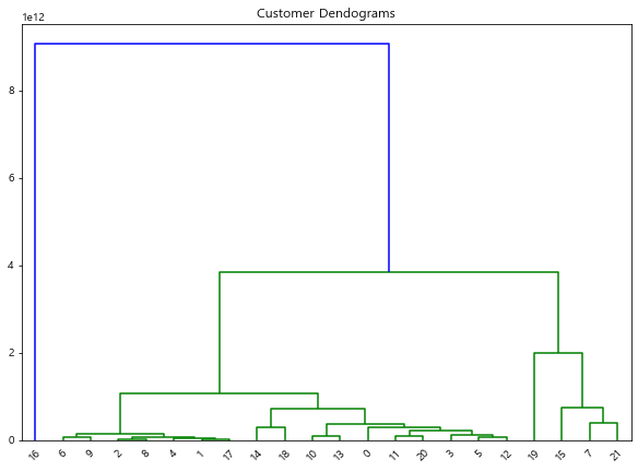
마지막으로 서비스업입니다. 서비스업은 약 20개의 업종이 존재하는데, 일반의원 업종을 제외하고 다른 업종들은 모두 하나의 그룹으로 묶인 것을 볼 수 있었습니다.
제가 진행해보았던 부분을 모두 작성해보았는데요.
군집 별 매출 분석이라거나, 예측 모델 만들기 등등 더 많은 것들을 추가적으로 해볼 수 있을 것 같아요.
부족한 글이지만 읽어주셔서 감사합니다. 😊